
To highlight cells with certain values in Excel, you use conditional formatting. This creates highlighted cells for certain content. In the example, you’ll learn how to highlight values in Excel easily.
Download the example here and follow along.
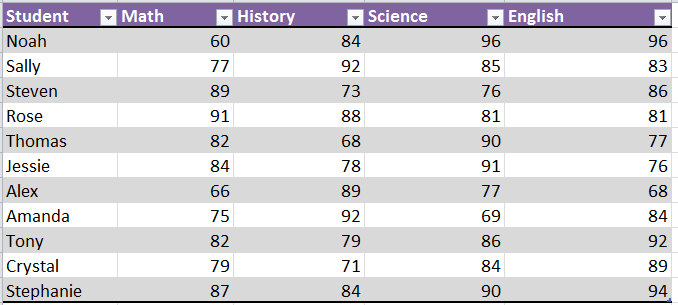
This example is of a grade book, and the goal is to highlight only the grades that are 90% and above.
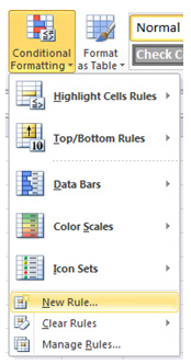
Begin by making sure you have selected the range of cells with only the values you desire. In the Home tab up top, select “Conditional Formatting” and choose “New Rule”.
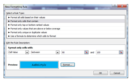
A dialog box will appear. Choose “Format only cells that contain” from this box.
In the boxes at the bottom of the dialog, there is the title “Format only cells with” and four drop down menus. Choose the following:
Cell value – between – 90 & 100.
Press the “Format” option and select a fill color for your highlight.
Press OK once you’ve finished.
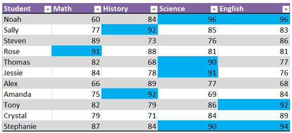
The spreadsheet will now generate cells with a different color background based on what you have previously entered as the value range containing scores that are 90% and above.
Related Templates:
- Conditional Formatting in Excel
- Highlight Rows in Excel
- How to Format Data with Excel
- Excel Dropdown Lists Tutorial
- Macros
View this offer while you wait!