

Macros in Excel let users automate tasks for them. In the example tutorial, you will learn how to combine values from two different columns to create a third column. The data is represented as first and last names.
Download the example tutorial.
First you must enable the use of Macros in Excel, so start by using the “Developer” toolbar. The “Developer” tool is not visible automatically, so follow these steps to get to it:
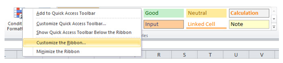
Right click in the top Ribbon then choose “Customize the Ribbon” from the options that appear.
In the dialog box, check “Developer” in the list on the right and press OK.

The Developer tab will now be visible for you to click in the Ribbon.
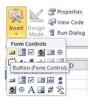
In the “Controls” group on the Developer toolbar, choose “Insert”, then select the first option.
Click anywhere inside the grid under the table in the spreadsheet area.
In this next step, name the Macro when the “Assign Macro” dialog box appears. In your example, it is already named as “Mybutton_click”.
Choose “New” and the Visual Basic code window will pop up.

After you enter “sub Mybutton_click()” press enter, and input the following:
x = 2
Do While Cells(x, 1).Value <> “”
Cells(x, 3).Value = Cells(x, 1).Value + ” ” + Cells(x, 2).Value
x = x + 1
Loop
This is the code that will loop through each Excel row, getting data from the first and second columns, and finally combining it in the third column to make a full name.
Press the Play button in the Visual Basic Editor and watch the results fill in the table automatically. You have now completed Macros.

Related Templates:
- Excel Dropdown Lists Tutorial
- Conditional Formatting in Excel
- How to Highlight Values in Excel
- Creating Pivot Tables in Excel
- How to Combine Two Names in Excel
View this offer while you wait!