
Applying conditional formatting in Excel is an easy and effective way to track progress on trigger-based actions.
Download the example and follow along to learn.
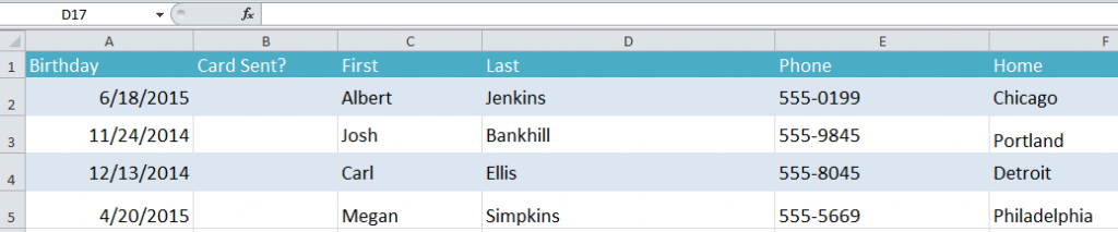
The example shows how Excel can track clients’ birthdays, and updates when a birthday has passed. As a trigger action, when the birthday passes, the formula in Excel will mark the “Card Sent” cell with a “yes” to indicate the change.
Creating this type of Excel sheet is easy. Use the example you downloaded to follow along.
Begin by selecting cells A2 through A5.
Choose “Conditional Formatting” in the Excel Ribbon Tool.
Next, choose “New Rule” from the drop down menu.
A dialog box will pop up when you do this. Choose “Use a formula to determine which cells to format”.
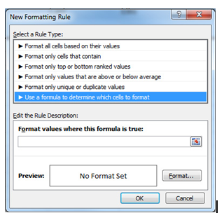
In this particular example, enter in the format value text box “=a2>TODAY()” and then click the “Format” button.
Click the top “Font” tab and select the color red, then make the font bold. Press OK to hide the dialog box.
The cell text will then be bold and red if the client’s birthday is on a future date.
IF statements in Excel
In this same example, go to cell B2 and input the following:
=IF(A2<TODAY(),”Y”,””)
This will tell Excel if the day has passed. If that is the case, then the cell will be marked as “Y” for yes, which will tell you if you sent the person a card for their birthday.
Finally, fill the formula through B5 using Excel’s fill handle so that all the cells in that column have the same formula. You can use this conditional formatting exercise for any Excel sheets that you want automatically updated according to dates or times.
Related Templates:
- How to Highlight Values in Excel
- How to Format Data with Excel
- Highlight Rows in Excel
- Creating Arrays in Excel
- Count Cells in Excel Formula
View this offer while you wait!