
Learn how to highlight rows in Excel with this function. If you are viewing, editing, or sorting through rows of data, it can be difficult to follow down the row and not accidentally look at the one below or above it. Highlight rows in Excel is an easy way to help you distinguish rows and view everything.
Download our example to try out highlighting rows yourself.
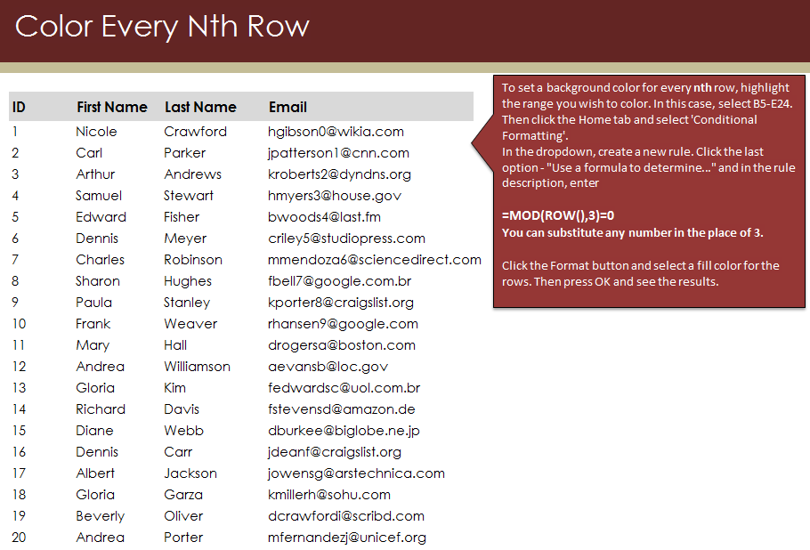
The example shows 20 entries in rows with names and emails. In this instance, you need to have a row highlighted after every two rows. To accomplish this, follow these steps:
Select cells B5 through E24 (click B5, hold Shift on the keyboard, and click E24) and then go to the top tab and choose “Conditional Formatting”.
The dropdown from that button will show the option “Create a new rule”. Click it and then choose the final option in the dialog box, “Use a formula to determine…” and under Rule Description, enter:
=MOD(ROW(),3)=0
Don’t click OK just yet! Hit “Format” and then choose the fill color you want for the rows. Then press OK and your results will be displayed.
You can change the “3” in the formula to a “2” if you want every other row highlighted, or “5” if you want to grab only every fifth piece of information. Changing the number to anything you want will work with this formula.
This function will help you when working with data or reading multiple rows.
To learn more Excel functions and formulas, see our tutorials and guides.
Related Templates:
- How to Highlight Values in Excel
- Conditional Formatting in Excel
- How to Prepend Text to Cells
- Excel Dropdown Lists Tutorial
- CTRL + Shift Selections
View this offer while you wait!