
Excel’s VLOOKUP function lets a user search the first column in a particular cell range and return data from a cell in the same row of that unique range.
This example is for you to follow along and learn how to use this function.
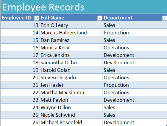
In this example, the VLOOKUP function is used to retrieve the full name or department name by using the employee ID.
The Syntax for VLOOKUP
VLOOKUP(lookup_value, table_array, col_index_num, [range_lookup])
Lookup_value – this is the value to search for
Table_array – Indicates the range of cells that contain the data desired.
Col_index_num – For the number of the particular column in table_array that you want a matching value from.
Range_lookup – (this is optional) decides if an exact or approximate match can be returned
VLOOKUP in the Example
In this example, you want to find out the first and last name of employee number 22 in the employee database.
Start by selecting cell A18.
From here, you start building the VLOOKUP function.
Since you know the value (employee number) to search for in the first column already, enter:
=VLOOKUP(22,
Next, enter the range of the data you want to search through.
=VLOOKUP(22,a3:c16,
Choose the number of the column that has the data you are searching for. “Full name” is in column two.
=VLOOKUP(22,a3:c16,2,
Since you need an exact match, enter:
=VLOOKUP(22,a3:c16,2, FALSE)
Now that you have the full formula, input it in cell A18. The result should be Martha Mackinnon if all was done correctly. You can replicate this VLOOKUP with your own spreadsheets.
Related Templates:
- Using the Index Match Function in Excel
- Using Exact Function
- How to Use the COUNTIF Function in Excel
- COUNT Between Numbers Template
- Get the Smallest Number in Excel Spreadsheet
View this offer while you wait!