
Have you ever wanted to change the look and appeal of your Excel spreadsheet? Maybe you want to write extensive messages, but find extending the columns in one row just makes the portions hard to deal with and impossible to print. The Concatenate feature in Excel is your way to take specific rows and combine them into one fluid cell, doing away with those pesky lines that chop up your information. The Concatenate function is the perfect way to write extended headers and messages without changing the cells of the rest of your document. Now you can keep that perfect printing structure and have a document that looks sharp and organized. Follow the instructions below to learn how to use the Concatenate feature.
How to Use the Concatenate Function in Excel
You can start by either following along with the free sample spreadsheet provided at the bottom of this page or by using your own spreadsheet and jumping right in.
- The only thing you need to enter into your SUM formula for the Concatenate is an ampersand (&).
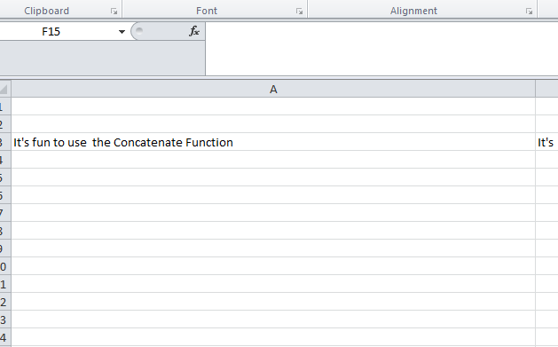
- For example, If you are following along in the sample spreadsheet, you will see a fully written message on the screen with and without the cell lines.
- If you want to combine your cells, all you need to do is click inside the cell you want to start your message and add this function into the formula bar.
- =B3&C3&D3&E3&F3&G3&H3
- Simply write the name of the cells you want to connect and link them with ampersand symbols in the formula bar.
- When you have successfully entered this function into your spreadsheet, your message or whatever you wanted to link together will be displayed into one fluid cell.
Using this function will allow you to create your spreadsheet with the sharp and organized look you’ve been craving.
Download: How to Use the Concatenate Function in Excel
Related Templates:
- How to Combine Two Names in Excel
- Using the Auto Fill Function in Excel
- Len Function Excel
- 3D SUM Function in Excel
- Using the ROUND Function in Excel
View this offer while you wait!