
Using the 3D SUM function is one of the best tools for calculating different numbers and figures through multiple tabs on your spreadsheet. For example, if you wanted to keep track of your monthly expenses over the next year and you have 12 tabs representing one month each, you’re going to look through a lot of data to get the exact information you need. This is where the 3D SUM function comes into play. If you need to receive a specific total for only one of the categories or items displayed on your spreadsheet, you would need to use this function to calculate the total through all 12 tabs to get the yearly sum. Instead of clicking through each tab and adding them on a calculator, just follow the steps below to use the 3D SUM function.
Steps to Use the 3D SUM Function in Excel
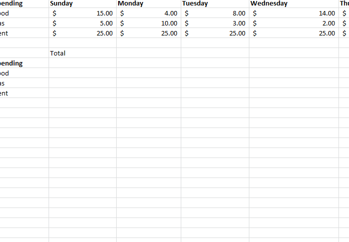
Start by downloading the free file located at the bottom of this page to follow the instructions below.
- After you have created or downloaded the spreadsheet you want to use this function for, you can begin to enter this formula for budget and sales tracking.
- Next, make a column where you can view your new total for the specific category or item.
- The 3D SUM function always has the same general structure, with just a few variables you need to change to make it fit your graph. If you are following along with the sample document, you’ll see the function structure.
- =SUM(‘Sheet1:Sheet7’!B2)
- After you have entered this formula into the document, in the designated “Total” column of the first tab, the function will give you the totals of all values in column B.
- To apply the 3D SUM function to your specific spreadsheet, simply change the “Sheet” variable to the title of your tabs and the B column to the column you want for your spreadsheet.
Download: 3D SUM Function in Excel
Related Templates:
- Using the Index Match Function in Excel
- Using the Auto Fill Function in Excel
- Using the ROUND Function in Excel
- How to Use the COUNTIF Function in Excel
- How to Use the Concatenate Function in Excel
View this offer while you wait!