
With Excel’s Pivot Table function, you can easily rearrange and view large amounts of data in an organized fashion. Just follow the steps below to learn how to use Pivot Tables.
Download the Pivot Table example to get started
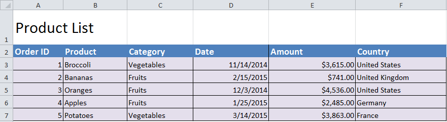
Start by clicking a cell.
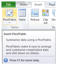
Click the “Insert” tab on the ribbon and choose PivotTable.
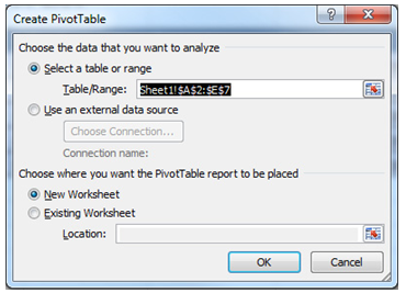
“Create PivotTable” dialog will appear. It will show the range of the pivot table that’s going to be created.
You can decide whether you want the PivotTable to be produced inside a new worksheet or the current sheet. Press OK once you’ve decided.
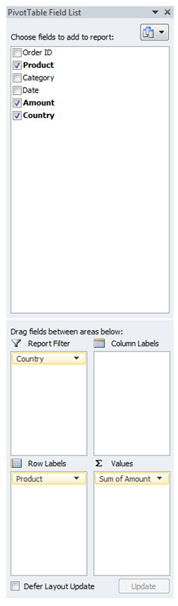
The list of fields will display on the screen. Choose the following options:
Product Field to Row Labels
Amount to Values area.
Country to Report Filters.
Check out your new PivotTable! It should look like this:
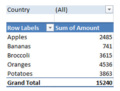
You now know how to use Excel’s Pivot Table function to manipulate data into easy to read fields.
Related Templates:
- Using the AUTOFILTER Function in Excel
- Filtering and Sorting with Excel
- Macros
- Pivot Point Calculator Excel
- Using the Index Match Function in Excel
View this offer while you wait!