
Learn to use the Excel Right Trim function with this guide. Get the last letters of a name or word with this easy formula. This function allows an Excel user to extract an indicated number of letters from a cell’s text starting from the last (most right) letter and going back. Learn how through our example.
Download the example here and follow along.
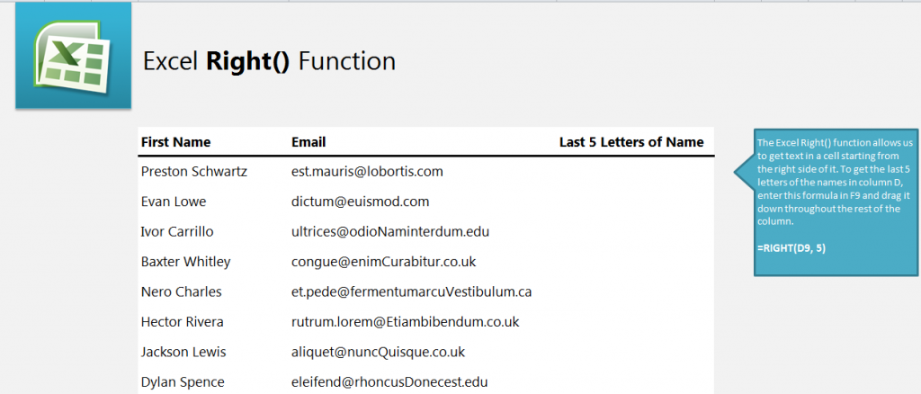
In the example you will be using column D to extract your information from and inserting it into column F. Start by selecting cell F9 and entering:
=RIGHT(D9, 5)
F9 will now be populated with “wartz”.
In the formula, D9 tells Excel where to get the information from, and the 5 shows how many letters you want returned.
To apply this formula to all the names, grab the corner of cell F9 and drag it down to F16. This will pull the last 5 letters of each name and insert them into their relating cells.
To experiment further with this example sheet, change the “5” to a new number and see the results. You can also use different amounts of letters on different cells. This function would be useful when organizing large amounts of data.
Eager to learn more about Excel functions and formulas? Visit our guides section.
Related Templates:
- Excel Left Function
- Len Function Excel
- How to Prepend Text to Cells
- Insert a Row in Excel
- Using the Auto Fill Function in Excel
View this offer while you wait!