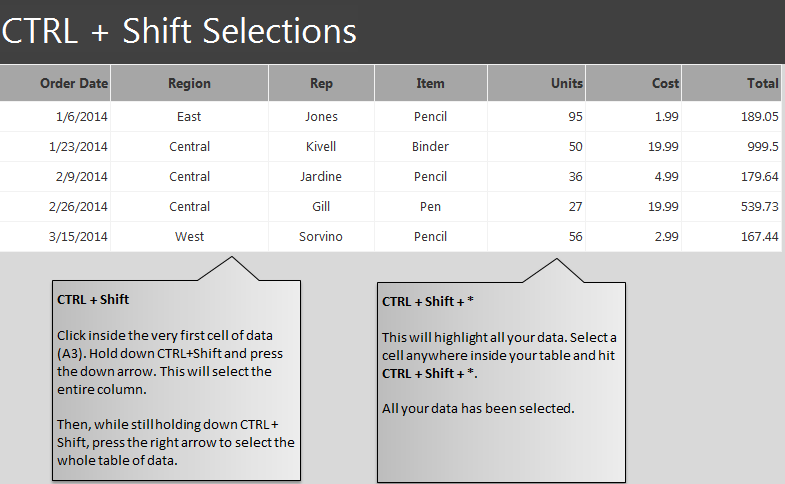
Learn to use CTRL + Shift selections in Excel worksheets to quickly and easily highlight sections of cells. This simple formula will make highlighting text a breeze. This formula can be used to apply colors, text fonts, or other changes to rows, columns, or isolated sections of Excel to quickly organize your worksheet.
Download our example worksheet to learn this formula.
Open the example worksheet and you will see populated columns and rows that you can use the CTRL + shift selection on. In the example, click in cell A3, then hold the CTRL and Shift buttons at the same time. From here, continue holding the buttons and press the down arrow on the keyboard to highlight the entire column.
To take it a step further, continue holding CTRL and shift and press the right arrow, which will select the whole table of data.
Try doing this from different cell starting points within the data sheet to see how you can utilize this.
To quickly highlight all of your entered data, select a cell anywhere within the populated sheet and then press CTRL, Shift, and * all at the same time. The whole data chart will be selected and you can then make mass changes easily.
Learn more about Excel’s functions and formulas in our guides section.
Related Templates:
- Highlight Rows in Excel
- Expense Budget Template
- Count Cells in Excel Formula
- Creating Arrays in Excel
- How to Prepend Text to Cells
View this offer while you wait!
